Page 372 - Applied Statistics with R

372 CHAPTER 15. COLLINEARITY

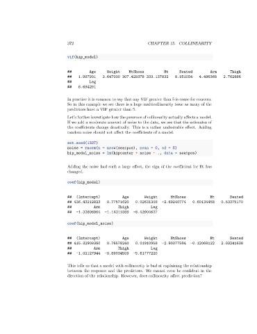
vif(hip_model)

## Age Weight HtShoes Ht Seated Arm Thigh
## 1.997931 3.647030 307.429378 333.137832 8.951054 4.496368 2.762886
## Leg
## 6.694291

In practice it is common to say that any VIF greater than 5 is cause for concern.
So in this example we see there is a huge multicollinearity issue as many of the
predictors have a VIF greater than 5.
Let’s further investigate how the presence of collinearity actually affects a model.
If we add a moderate amount of noise to the data, we see that the estimates of
the coefficients change drastically. This is a rather undesirable effect. Adding
random noise should not affect the coefficients of a model.

set.seed(1337)
noise = rnorm(n = nrow(seatpos), mean = 0, sd = 5)
hip_model_noise = lm(hipcenter + noise ~ ., data = seatpos)

Adding the noise had such a large effect, the sign of the coefficient for Ht has
changed.

coef(hip_model)

## (Intercept) Age Weight HtShoes Ht Seated
## 436.43212823 0.77571620 0.02631308 -2.69240774 0.60134458 0.53375170
## Arm Thigh Leg
## -1.32806864 -1.14311888 -6.43904627

coef(hip_model_noise)

## (Intercept) Age Weight HtShoes Ht Seated
## 415.32909380 0.76578240 0.01910958 -2.90377584 -0.12068122 2.03241638
## Arm Thigh Leg
## -1.02127944 -0.89034509 -5.61777220

This tells us that a model with collinearity is bad at explaining the relationship
between the response and the predictors. We cannot even be confident in the
direction of the relationship. However, does collinearity affect prediction?