Page 109 - Python Data Science Handbook

In[23]: plt.scatter(X[:, 0], X[:, 1], s=100)
# draw lines from each point to its two nearest neighbors
K = 2
for i in range(X.shape[0]):
for j in nearest_partition[i, :K+1]:
# plot a line from X[i] to X[j]
# use some zip magic to make it happen:
plt.plot(*zip(X[j], X[i]), color='black')

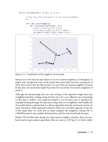
Figure 2-11. Visualization of the neighbors of each point

Each point in the plot has lines drawn to its two nearest neighbors. At first glance, it
might seem strange that some of the points have more than two lines coming out of
them: this is due to the fact that if point A is one of the two nearest neighbors of point
B, this does not necessarily imply that point B is one of the two nearest neighbors of
point A.
Although the broadcasting and row-wise sorting of this approach might seem less
straightforward than writing a loop, it turns out to be a very efficient way of operating
on this data in Python. You might be tempted to do the same type of operation by
manually looping through the data and sorting each set of neighbors individually, but
this would almost certainly lead to a slower algorithm than the vectorized version we
used. The beauty of this approach is that it’s written in a way that’s agnostic to the size
of the input data: we could just as easily compute the neighbors among 100 or
1,000,000 points in any number of dimensions, and the code would look the same.
Finally, I’ll note that when doing very large nearest-neighbor searches, there are tree-
based and/or approximate algorithms that can scale as ᇭ N log N or better rather

Sorting Arrays | 91