Page 107 - Python Data Science Handbook

points on a two-dimensional plane. Using the standard convention, we’ll arrange
these in a 10×2 array:

In[14]: X = rand.rand(10, 2)
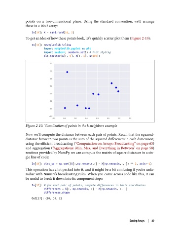
To get an idea of how these points look, let’s quickly scatter plot them (Figure 2-10):

In[15]: %matplotlib inline
import matplotlib.pyplot as plt
import seaborn; seaborn.set() # Plot styling
plt.scatter(X[:, 0], X[:, 1], s=100);

Figure 2-10. Visualization of points in the k-neighbors example

Now we’ll compute the distance between each pair of points. Recall that the squared-
distance between two points is the sum of the squared differences in each dimension;
using the efficient broadcasting (“Computation on Arrays: Broadcasting” on page 63)
and aggregation (“Aggregations: Min, Max, and Everything in Between” on page 58)
routines provided by NumPy, we can compute the matrix of square distances in a sin‐
gle line of code:
In[16]: dist_sq = np.sum((X[:,np.newaxis,:] - X[np.newaxis,:,:]) ** 2, axis=-1)
This operation has a lot packed into it, and it might be a bit confusing if you’re unfa‐
miliar with NumPy’s broadcasting rules. When you come across code like this, it can
be useful to break it down into its component steps:

In[17]: # for each pair of points, compute differences in their coordinates
differences = X[:, np.newaxis, :] - X[np.newaxis, :, :]
differences.shape
Out[17]: (10, 10, 2)

Sorting Arrays | 89