Page 108 - Python Data Science Handbook

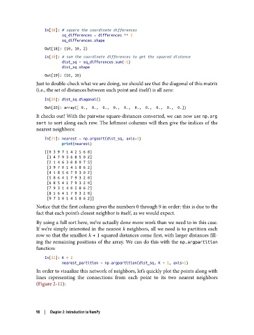
In[18]: # square the coordinate differences
sq_differences = differences ** 2
sq_differences.shape
Out[18]: (10, 10, 2)

In[19]: # sum the coordinate differences to get the squared distance
dist_sq = sq_differences.sum(-1)
dist_sq.shape
Out[19]: (10, 10)
Just to double-check what we are doing, we should see that the diagonal of this matrix
(i.e., the set of distances between each point and itself) is all zero:

In[20]: dist_sq.diagonal()
Out[20]: array([ 0., 0., 0., 0., 0., 0., 0., 0., 0., 0.])
It checks out! With the pairwise square-distances converted, we can now use np.arg
sort to sort along each row. The leftmost columns will then give the indices of the
nearest neighbors:

In[21]: nearest = np.argsort(dist_sq, axis=1)
print(nearest)
[[0 3 9 7 1 4 2 5 6 8]
[1 4 7 9 3 6 8 5 0 2]
[2 1 4 6 3 0 8 9 7 5]
[3 9 7 0 1 4 5 8 6 2]
[4 1 8 5 6 7 9 3 0 2]
[5 8 6 4 1 7 9 3 2 0]
[6 8 5 4 1 7 9 3 2 0]
[7 9 3 1 4 0 5 8 6 2]
[8 5 6 4 1 7 9 3 2 0]
[9 7 3 0 1 4 5 8 6 2]]
Notice that the first column gives the numbers 0 through 9 in order: this is due to the
fact that each point’s closest neighbor is itself, as we would expect.
By using a full sort here, we’ve actually done more work than we need to in this case.
If we’re simply interested in the nearest k neighbors, all we need is to partition each
row so that the smallest k + 1 squared distances come first, with larger distances fill‐
ing the remaining positions of the array. We can do this with the np.argpartition
function:

In[22]: K = 2
nearest_partition = np.argpartition(dist_sq, K + 1, axis=1)
In order to visualize this network of neighbors, let’s quickly plot the points along with
lines representing the connections from each point to its two nearest neighbors
(Figure 2-11):

90 | Chapter 2: Introduction to NumPy