Page 183 - Python Data Science Handbook

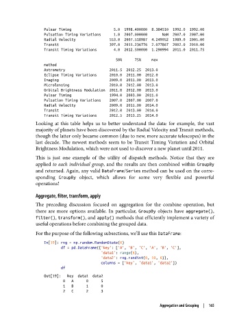
Pulsar Timing 5.0 1998.400000 8.384510 1992.0 1992.00
Pulsation Timing Variations 1.0 2007.000000 NaN 2007.0 2007.00
Radial Velocity 553.0 2007.518987 4.249052 1989.0 2005.00
Transit 397.0 2011.236776 2.077867 2002.0 2010.00
Transit Timing Variations 4.0 2012.500000 1.290994 2011.0 2011.75
50% 75% max
method
Astrometry 2011.5 2012.25 2013.0
Eclipse Timing Variations 2010.0 2011.00 2012.0
Imaging 2009.0 2011.00 2013.0
Microlensing 2010.0 2012.00 2013.0
Orbital Brightness Modulation 2011.0 2012.00 2013.0
Pulsar Timing 1994.0 2003.00 2011.0
Pulsation Timing Variations 2007.0 2007.00 2007.0
Radial Velocity 2009.0 2011.00 2014.0
Transit 2012.0 2013.00 2014.0
Transit Timing Variations 2012.5 2013.25 2014.0
Looking at this table helps us to better understand the data: for example, the vast
majority of planets have been discovered by the Radial Velocity and Transit methods,
though the latter only became common (due to new, more accurate telescopes) in the
last decade. The newest methods seem to be Transit Timing Variation and Orbital
Brightness Modulation, which were not used to discover a new planet until 2011.

This is just one example of the utility of dispatch methods. Notice that they are
applied to each individual group, and the results are then combined within GroupBy
and returned. Again, any valid DataFrame/Series method can be used on the corre‐
sponding GroupBy object, which allows for some very flexible and powerful
operations!

Aggregate, filter, transform, apply

The preceding discussion focused on aggregation for the combine operation, but
there are more options available. In particular, GroupBy objects have aggregate(),
filter(), transform(), and apply() methods that efficiently implement a variety of
useful operations before combining the grouped data.
For the purpose of the following subsections, we’ll use this DataFrame:

In[19]: rng = np.random.RandomState(0)
df = pd.DataFrame({'key': ['A', 'B', 'C', 'A', 'B', 'C'],
'data1': range(6),
'data2': rng.randint(0, 10, 6)},
columns = ['key', 'data1', 'data2'])
df
Out[19]: key data1 data2
0 A 0 5
1 B 1 0
2 C 2 3

Aggregation and Grouping | 165