Page 178 - Python Data Science Handbook

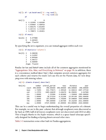
In[7]: df = pd.DataFrame({'A': rng.rand(5),
'B': rng.rand(5)})
df
Out[7]: A B
0 0.155995 0.020584
1 0.058084 0.969910
2 0.866176 0.832443
3 0.601115 0.212339
4 0.708073 0.181825
In[8]: df.mean()
Out[8]: A 0.477888
B 0.443420
dtype: float64
By specifying the axis argument, you can instead aggregate within each row:

In[9]: df.mean(axis='columns')
Out[9]: 0 0.088290
1 0.513997
2 0.849309
3 0.406727
4 0.444949
dtype: float64
Pandas Series and DataFrames include all of the common aggregates mentioned in
“Aggregations: Min, Max, and Everything in Between” on page 58; in addition, there
is a convenience method describe() that computes several common aggregates for
each column and returns the result. Let’s use this on the Planets data, for now drop‐
ping rows with missing values:

In[10]: planets.dropna().describe()
Out[10]: number orbital_period mass distance year
count 498.00000 498.000000 498.000000 498.000000 498.000000
mean 1.73494 835.778671 2.509320 52.068213 2007.377510
std 1.17572 1469.128259 3.636274 46.596041 4.167284
min 1.00000 1.328300 0.003600 1.350000 1989.000000
25% 1.00000 38.272250 0.212500 24.497500 2005.000000
50% 1.00000 357.000000 1.245000 39.940000 2009.000000
75% 2.00000 999.600000 2.867500 59.332500 2011.000000
max 6.00000 17337.500000 25.000000 354.000000 2014.000000
This can be a useful way to begin understanding the overall properties of a dataset.
For example, we see in the year column that although exoplanets were discovered as
far back as 1989, half of all known exoplanets were not discovered until 2010 or after.
This is largely thanks to the Kepler mission, which is a space-based telescope specifi‐
cally designed for finding eclipsing planets around other stars.

Table 3-3 summarizes some other built-in Pandas aggregations.

160 | Chapter 3: Data Manipulation with Pandas