Page 193 - Python Data Science Handbook

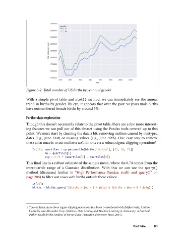
Figure 3-2. Total number of US births by year and gender

With a simple pivot table and plot() method, we can immediately see the annual
trend in births by gender. By eye, it appears that over the past 50 years male births
have outnumbered female births by around 5%.

Further data exploration
Though this doesn’t necessarily relate to the pivot table, there are a few more interest‐
ing features we can pull out of this dataset using the Pandas tools covered up to this
point. We must start by cleaning the data a bit, removing outliers caused by mistyped
dates (e.g., June 31st) or missing values (e.g., June 99th). One easy way to remove
these all at once is to cut outliers; we’ll do this via a robust sigma-clipping operation: 1
In[15]: quartiles = np.percentile(births['births'], [25, 50, 75])
mu = quartiles[1]
sig = 0.74 * (quartiles[2] - quartiles[0])
This final line is a robust estimate of the sample mean, where the 0.74 comes from the
interquartile range of a Gaussian distribution. With this we can use the query()
method (discussed further in “High-Performance Pandas: eval() and query()” on
page 208) to filter out rows with births outside these values:

In[16]:
births = births.query('(births > @mu - 5 * @sig) & (births < @mu + 5 * @sig)')

1 You can learn more about sigma-clipping operations in a book I coauthored with Željko Ivezić, Andrew J.
Connolly, and Alexander Gray: Statistics, Data Mining, and Machine Learning in Astronomy: A Practical
Python Guide for the Analysis of Survey Data (Princeton University Press, 2014).

Pivot Tables | 175