Page 190 - Python Data Science Handbook

gradient favors both women and higher classes. First-class women survived with near
certainty (hi, Rose!), while only one in ten third-class men survived (sorry, Jack!).

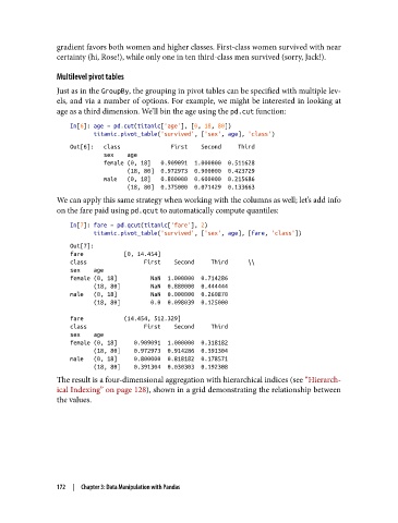
Multilevel pivot tables

Just as in the GroupBy, the grouping in pivot tables can be specified with multiple lev‐
els, and via a number of options. For example, we might be interested in looking at
age as a third dimension. We’ll bin the age using the pd.cut function:
In[6]: age = pd.cut(titanic['age'], [0, 18, 80])
titanic.pivot_table('survived', ['sex', age], 'class')
Out[6]: class First Second Third
sex age
female (0, 18] 0.909091 1.000000 0.511628
(18, 80] 0.972973 0.900000 0.423729
male (0, 18] 0.800000 0.600000 0.215686
(18, 80] 0.375000 0.071429 0.133663
We can apply this same strategy when working with the columns as well; let’s add info
on the fare paid using pd.qcut to automatically compute quantiles:

In[7]: fare = pd.qcut(titanic['fare'], 2)
titanic.pivot_table('survived', ['sex', age], [fare, 'class'])
Out[7]:
fare [0, 14.454]
class First Second Third \\
sex age
female (0, 18] NaN 1.000000 0.714286
(18, 80] NaN 0.880000 0.444444
male (0, 18] NaN 0.000000 0.260870
(18, 80] 0.0 0.098039 0.125000

fare (14.454, 512.329]
class First Second Third
sex age
female (0, 18] 0.909091 1.000000 0.318182
(18, 80] 0.972973 0.914286 0.391304
male (0, 18] 0.800000 0.818182 0.178571
(18, 80] 0.391304 0.030303 0.192308
The result is a four-dimensional aggregation with hierarchical indices (see “Hierarch‐
ical Indexing” on page 128), shown in a grid demonstrating the relationship between
the values.

172 | Chapter 3: Data Manipulation with Pandas