Page 310 - Python Data Science Handbook

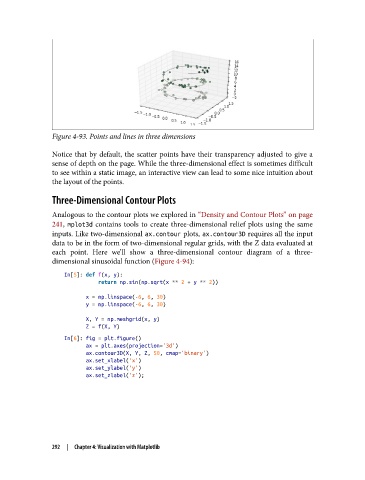
Figure 4-93. Points and lines in three dimensions

Notice that by default, the scatter points have their transparency adjusted to give a
sense of depth on the page. While the three-dimensional effect is sometimes difficult
to see within a static image, an interactive view can lead to some nice intuition about
the layout of the points.

Three-Dimensional Contour Plots

Analogous to the contour plots we explored in “Density and Contour Plots” on page
241, mplot3d contains tools to create three-dimensional relief plots using the same
inputs. Like two-dimensional ax.contour plots, ax.contour3D requires all the input
data to be in the form of two-dimensional regular grids, with the Z data evaluated at
each point. Here we’ll show a three-dimensional contour diagram of a three-
dimensional sinusoidal function (Figure 4-94):

In[5]: def f(x, y):
return np.sin(np.sqrt(x ** 2 + y ** 2))

x = np.linspace(-6, 6, 30)
y = np.linspace(-6, 6, 30)
X, Y = np.meshgrid(x, y)
Z = f(X, Y)
In[6]: fig = plt.figure()
ax = plt.axes(projection='3d')
ax.contour3D(X, Y, Z, 50, cmap='binary')
ax.set_xlabel('x')
ax.set_ylabel('y')
ax.set_zlabel('z');

292 | Chapter 4: Visualization with Matplotlib