Page 313 - Python Data Science Handbook

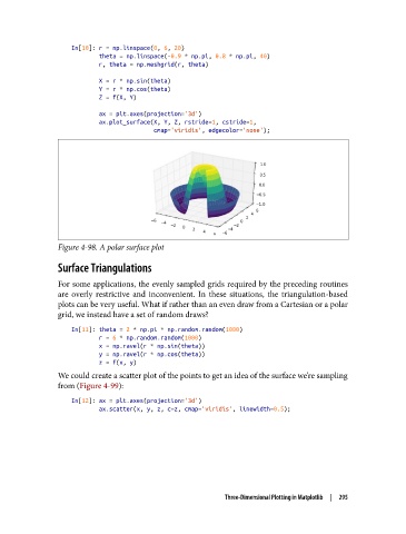
In[10]: r = np.linspace(0, 6, 20)
theta = np.linspace(-0.9 * np.pi, 0.8 * np.pi, 40)
r, theta = np.meshgrid(r, theta)

X = r * np.sin(theta)
Y = r * np.cos(theta)
Z = f(X, Y)

ax = plt.axes(projection='3d')
ax.plot_surface(X, Y, Z, rstride=1, cstride=1,
cmap='viridis', edgecolor='none');

Figure 4-98. A polar surface plot

Surface Triangulations

For some applications, the evenly sampled grids required by the preceding routines
are overly restrictive and inconvenient. In these situations, the triangulation-based
plots can be very useful. What if rather than an even draw from a Cartesian or a polar
grid, we instead have a set of random draws?
In[11]: theta = 2 * np.pi * np.random.random(1000)
r = 6 * np.random.random(1000)
x = np.ravel(r * np.sin(theta))
y = np.ravel(r * np.cos(theta))
z = f(x, y)
We could create a scatter plot of the points to get an idea of the surface we’re sampling
from (Figure 4-99):

In[12]: ax = plt.axes(projection='3d')
ax.scatter(x, y, z, c=z, cmap='viridis', linewidth=0.5);

Three-Dimensional Plotting in Matplotlib | 295