Page 347 - Python Data Science Handbook

Also surprisingly, the 80-year-old women seem to outperform everyone in terms of
their split time. This is probably due to the fact that we’re estimating the distribution
from small numbers, as there are only a handful of runners in that range:
In[38]: (data.age > 80).sum()
Out[38]: 7
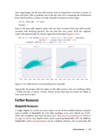
Back to the men with negative splits: who are these runners? Does this split fraction
correlate with finishing quickly? We can plot this very easily. We’ll use regplot,
which will automatically fit a linear regression to the data (Figure 4-132):

In[37]: g = sns.lmplot('final_sec', 'split_frac', col='gender', data=data,
markers=".", scatter_kws=dict(color='c'))
g.map(plt.axhline, y=0.1, color="k", ls=":");

Figure 4-132. Split fraction versus finishing time by gender

Apparently the people with fast splits are the elite runners who are finishing within
~15,000 seconds, or about 4 hours. People slower than that are much less likely to
have a fast second split.

Further Resources

Matplotlib Resources

A single chapter in a book can never hope to cover all the available features and plot
types available in Matplotlib. As with other packages we’ve seen, liberal use of IPy‐
thon’s tab-completion and help functions (see “Help and Documentation in IPython”
on page 3) can be very helpful when you’re exploring Matplotlib’s API. In addition,
Matplotlib’s online documentation can be a helpful reference. See in particular the

Further Resources | 329