Page 368 - Python Data Science Handbook

In[10]: model.coef_
Out[10]: array([ 1.9776566])
In[11]: model.intercept_
Out[11]: -0.90331072553111635
These two parameters represent the slope and intercept of the simple linear fit to
the data. Comparing to the data definition, we see that they are very close to the
input slope of 2 and intercept of –1.
One question that frequently comes up regards the uncertainty in such internal
model parameters. In general, Scikit-Learn does not provide tools to draw con‐
clusions from internal model parameters themselves: interpreting model parame‐
ters is much more a statistical modeling question than a machine learning
question. Machine learning rather focuses on what the model predicts. If you
would like to dive into the meaning of fit parameters within the model, other
tools are available, including the StatsModels Python package.
5. Predict labels for unknown data.
Once the model is trained, the main task of supervised machine learning is to
evaluate it based on what it says about new data that was not part of the training
set. In Scikit-Learn, we can do this using the predict() method. For the sake of
this example, our “new data” will be a grid of x values, and we will ask what y
values the model predicts:
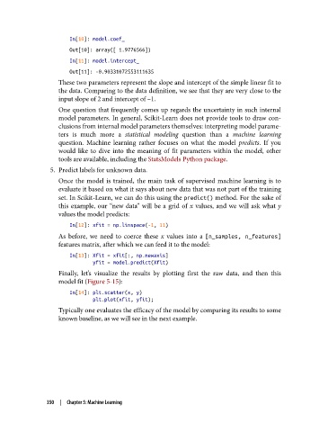
In[12]: xfit = np.linspace(-1, 11)
As before, we need to coerce these x values into a [n_samples, n_features]
features matrix, after which we can feed it to the model:
In[13]: Xfit = xfit[:, np.newaxis]
yfit = model.predict(Xfit)
Finally, let’s visualize the results by plotting first the raw data, and then this
model fit (Figure 5-15):
In[14]: plt.scatter(x, y)
plt.plot(xfit, yfit);
Typically one evaluates the efficacy of the model by comparing its results to some
known baseline, as we will see in the next example.

350 | Chapter 5: Machine Learning