Page 370 - Python Data Science Handbook

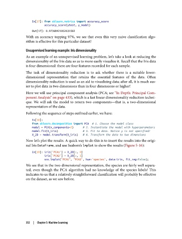
In[17]: from sklearn.metrics import accuracy_score
accuracy_score(ytest, y_model)
Out[17]: 0.97368421052631582
With an accuracy topping 97%, we see that even this very naive classification algo‐
rithm is effective for this particular dataset!

Unsupervised learning example: Iris dimensionality

As an example of an unsupervised learning problem, let’s take a look at reducing the
dimensionality of the Iris data so as to more easily visualize it. Recall that the Iris data
is four dimensional: there are four features recorded for each sample.
The task of dimensionality reduction is to ask whether there is a suitable lower-
dimensional representation that retains the essential features of the data. Often
dimensionality reduction is used as an aid to visualizing data; after all, it is much eas‐
ier to plot data in two dimensions than in four dimensions or higher!
Here we will use principal component analysis (PCA; see “In Depth: Principal Com‐
ponent Analysis” on page 433), which is a fast linear dimensionality reduction techni‐
que. We will ask the model to return two components—that is, a two-dimensional
representation of the data.
Following the sequence of steps outlined earlier, we have:

In[18]:
from sklearn.decomposition import PCA # 1. Choose the model class
model = PCA(n_components=2) # 2. Instantiate the model with hyperparameters
model.fit(X_iris) # 3. Fit to data. Notice y is not specified!
X_2D = model.transform(X_iris) # 4. Transform the data to two dimensions
Now let’s plot the results. A quick way to do this is to insert the results into the origi‐
nal Iris DataFrame, and use Seaborn’s lmplot to show the results (Figure 5-16):

In[19]: iris['PCA1'] = X_2D[:, 0]
iris['PCA2'] = X_2D[:, 1]
sns.lmplot("PCA1", "PCA2", hue='species', data=iris, fit_reg=False);
We see that in the two-dimensional representation, the species are fairly well separa‐
ted, even though the PCA algorithm had no knowledge of the species labels! This
indicates to us that a relatively straightforward classification will probably be effective
on the dataset, as we saw before.

352 | Chapter 5: Machine Learning