Page 376 - Python Data Science Handbook

This shows us where the mislabeled points tend to be: for example, a large number of
twos here are misclassified as either ones or eights. Another way to gain intuition into
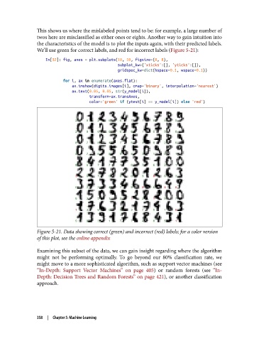
the characteristics of the model is to plot the inputs again, with their predicted labels.
We’ll use green for correct labels, and red for incorrect labels (Figure 5-21):

In[32]: fig, axes = plt.subplots(10, 10, figsize=(8, 8),
subplot_kw={'xticks':[], 'yticks':[]},
gridspec_kw=dict(hspace=0.1, wspace=0.1))

for i, ax in enumerate(axes.flat):
ax.imshow(digits.images[i], cmap='binary', interpolation='nearest')
ax.text(0.05, 0.05, str(y_model[i]),
transform=ax.transAxes,
color='green' if (ytest[i] == y_model[i]) else 'red')

Figure 5-21. Data showing correct (green) and incorrect (red) labels; for a color version
of this plot, see the online appendix

Examining this subset of the data, we can gain insight regarding where the algorithm
might not be performing optimally. To go beyond our 80% classification rate, we
might move to a more sophisticated algorithm, such as support vector machines (see
“In-Depth: Support Vector Machines” on page 405) or random forests (see “In-
Depth: Decision Trees and Random Forests” on page 421), or another classification
approach.

358 | Chapter 5: Machine Learning