Page 401 - Python Data Science Handbook

Bayesian Classification

Naive Bayes classifiers are built on Bayesian classification methods. These rely on
Bayes’s theorem, which is an equation describing the relationship of conditional
probabilities of statistical quantities. In Bayesian classification, we’re interested in
finding the probability of a label given some observed features, which we can write as
P L features . Bayes’s theorem tells us how to express this in terms of quantities we
can compute more directly:

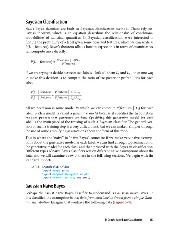
P L features = P features L P L
P features

If we are trying to decide between two labels—let’s call them L and L —then one way
1
2
to make this decision is to compute the ratio of the posterior probabilities for each
label:

P L 1 features P features L 1 P L 1
P L 1 features = P features L 2 P L 2

All we need now is some model by which we can compute P features L for each
i
label. Such a model is called a generative model because it specifies the hypothetical
random process that generates the data. Specifying this generative model for each
label is the main piece of the training of such a Bayesian classifier. The general ver‐
sion of such a training step is a very difficult task, but we can make it simpler through
the use of some simplifying assumptions about the form of this model.
This is where the “naive” in “naive Bayes” comes in: if we make very naive assump‐
tions about the generative model for each label, we can find a rough approximation of
the generative model for each class, and then proceed with the Bayesian classification.
Different types of naive Bayes classifiers rest on different naive assumptions about the
data, and we will examine a few of these in the following sections. We begin with the
standard imports:

In[1]: %matplotlib inline
import numpy as np
import matplotlib.pyplot as plt
import seaborn as sns; sns.set()
Gaussian Naive Bayes

Perhaps the easiest naive Bayes classifier to understand is Gaussian naive Bayes. In
this classifier, the assumption is that data from each label is drawn from a simple Gaus‐
sian distribution. Imagine that you have the following data (Figure 5-38):

In Depth: Naive Bayes Classification | 383