Page 499 - Python Data Science Handbook

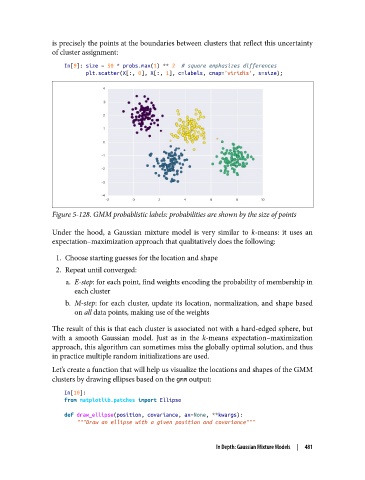
is precisely the points at the boundaries between clusters that reflect this uncertainty
of cluster assignment:

In[9]: size = 50 * probs.max(1) ** 2 # square emphasizes differences
plt.scatter(X[:, 0], X[:, 1], c=labels, cmap='viridis', s=size);

Figure 5-128. GMM probablistic labels: probabilities are shown by the size of points

Under the hood, a Gaussian mixture model is very similar to k-means: it uses an
expectation–maximization approach that qualitatively does the following:

1. Choose starting guesses for the location and shape
2. Repeat until converged:
a. E-step: for each point, find weights encoding the probability of membership in
each cluster
b. M-step: for each cluster, update its location, normalization, and shape based
on all data points, making use of the weights

The result of this is that each cluster is associated not with a hard-edged sphere, but
with a smooth Gaussian model. Just as in the k-means expectation–maximization
approach, this algorithm can sometimes miss the globally optimal solution, and thus
in practice multiple random initializations are used.

Let’s create a function that will help us visualize the locations and shapes of the GMM
clusters by drawing ellipses based on the gmm output:

In[10]:
from matplotlib.patches import Ellipse

def draw_ellipse(position, covariance, ax=None, **kwargs):
"""Draw an ellipse with a given position and covariance"""

In Depth: Gaussian Mixture Models | 481