Page 494 - Python Data Science Handbook

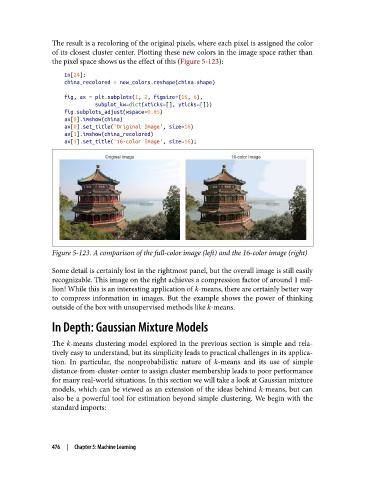
The result is a recoloring of the original pixels, where each pixel is assigned the color
of its closest cluster center. Plotting these new colors in the image space rather than
the pixel space shows us the effect of this (Figure 5-123):
In[24]:
china_recolored = new_colors.reshape(china.shape)
fig, ax = plt.subplots(1, 2, figsize=(16, 6),
subplot_kw=dict(xticks=[], yticks=[]))
fig.subplots_adjust(wspace=0.05)
ax[0].imshow(china)
ax[0].set_title('Original Image', size=16)
ax[1].imshow(china_recolored)
ax[1].set_title('16-color Image', size=16);

Figure 5-123. A comparison of the full-color image (left) and the 16-color image (right)

Some detail is certainly lost in the rightmost panel, but the overall image is still easily
recognizable. This image on the right achieves a compression factor of around 1 mil‐
lion! While this is an interesting application of k-means, there are certainly better way
to compress information in images. But the example shows the power of thinking
outside of the box with unsupervised methods like k-means.

In Depth: Gaussian Mixture Models

The k-means clustering model explored in the previous section is simple and rela‐
tively easy to understand, but its simplicity leads to practical challenges in its applica‐
tion. In particular, the nonprobabilistic nature of k-means and its use of simple
distance-from-cluster-center to assign cluster membership leads to poor performance
for many real-world situations. In this section we will take a look at Gaussian mixture
models, which can be viewed as an extension of the ideas behind k-means, but can
also be a powerful tool for estimation beyond simple clustering. We begin with the
standard imports:

476 | Chapter 5: Machine Learning