Page 495 - Python Data Science Handbook

In[1]: %matplotlib inline
import matplotlib.pyplot as plt
import seaborn as sns; sns.set()
import numpy as np
Motivating GMM: Weaknesses of k-Means

Let’s take a look at some of the weaknesses of k-means and think about how we might
improve the cluster model. As we saw in the previous section, given simple, well-
separated data, k-means finds suitable clustering results.
For example, if we have simple blobs of data, the k-means algorithm can quickly label
those clusters in a way that closely matches what we might do by eye (Figure 5-124):
In[2]: # Generate some data
from sklearn.datasets.samples_generator import make_blobs
X, y_true = make_blobs(n_samples=400, centers=4,
cluster_std=0.60, random_state=0)
X = X[:, ::-1] # flip axes for better plotting
In[3]: # Plot the data with k-means labels
from sklearn.cluster import KMeans
kmeans = KMeans(4, random_state=0)
labels = kmeans.fit(X).predict(X)
plt.scatter(X[:, 0], X[:, 1], c=labels, s=40, cmap='viridis');

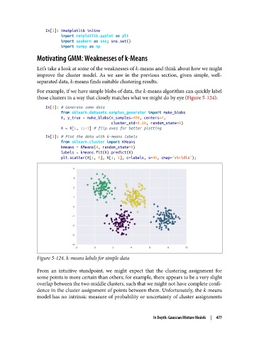
Figure 5-124. k-means labels for simple data

From an intuitive standpoint, we might expect that the clustering assignment for
some points is more certain than others; for example, there appears to be a very slight
overlap between the two middle clusters, such that we might not have complete confi‐
dence in the cluster assignment of points between them. Unfortunately, the k-means
model has no intrinsic measure of probability or uncertainty of cluster assignments

In Depth: Gaussian Mixture Models | 477