Page 517 - Python Data Science Handbook

# Get matrices/arrays of species IDs and locations
latlon = np.vstack([data.train['dd lat'],
data.train['dd long']]).T
species = np.array([d.decode('ascii').startswith('micro')
for d in data.train['species']], dtype='int')
With this data loaded, we can use the Basemap toolkit (mentioned previously in
“Geographic Data with Basemap” on page 298) to plot the observed locations of these
two species on the map of South America (Figure 5-146):

In[14]: from mpl_toolkits.basemap import Basemap
from sklearn.datasets.species_distributions import construct_grids
xgrid, ygrid = construct_grids(data)

# plot coastlines with Basemap
m = Basemap(projection='cyl', resolution='c',
llcrnrlat=ygrid.min(), urcrnrlat=ygrid.max(),
llcrnrlon=xgrid.min(), urcrnrlon=xgrid.max())
m.drawmapboundary(fill_color='#DDEEFF')
m.fillcontinents(color='#FFEEDD')
m.drawcoastlines(color='gray', zorder=2)
m.drawcountries(color='gray', zorder=2)

# plot locations
m.scatter(latlon[:, 1], latlon[:, 0], zorder=3,
c=species, cmap='rainbow', latlon=True);

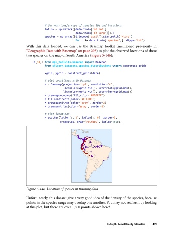
Figure 5-146. Location of species in training data

Unfortunately, this doesn’t give a very good idea of the density of the species, because
points in the species range may overlap one another. You may not realize it by looking
at this plot, but there are over 1,600 points shown here!

In-Depth: Kernel Density Estimation | 499