Page 519 - Python Data Science Handbook

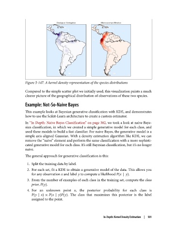
Figure 5-147. A kernel density representation of the species distributions

Compared to the simple scatter plot we initially used, this visualization paints a much
clearer picture of the geographical distribution of observations of these two species.

Example: Not-So-Naive Bayes

This example looks at Bayesian generative classification with KDE, and demonstrates
how to use the Scikit-Learn architecture to create a custom estimator.

In “In Depth: Naive Bayes Classification” on page 382, we took a look at naive Baye‐
sian classification, in which we created a simple generative model for each class, and
used these models to build a fast classifier. For naive Bayes, the generative model is a
simple axis-aligned Gaussian. With a density estimation algorithm like KDE, we can
remove the “naive” element and perform the same classification with a more sophisti‐
cated generative model for each class. It’s still Bayesian classification, but it’s no longer
naive.
The general approach for generative classification is this:

1. Split the training data by label.
2. For each set, fit a KDE to obtain a generative model of the data. This allows you
for any observation x and label y to compute a likelihood P x y .
3. From the number of examples of each class in the training set, compute the class
prior, P y .

4. For an unknown point x, the posterior probability for each class is
P y x ֣ P x y P y . The class that maximizes this posterior is the label
assigned to the point.

In-Depth: Kernel Density Estimation | 501