Page 525 - Python Data Science Handbook

4. Normalize the histograms in each cell by comparing to the block of neighboring
cells. This further suppresses the effect of illumination across the image.
5. Construct a one-dimensional feature vector from the information in each cell.

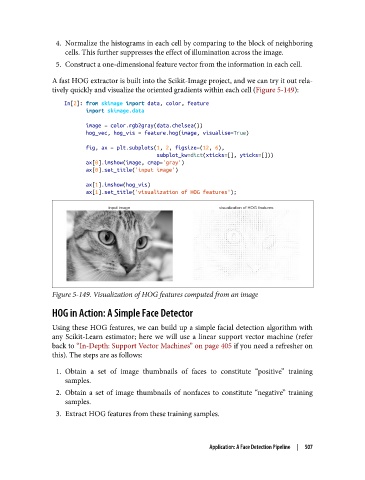
A fast HOG extractor is built into the Scikit-Image project, and we can try it out rela‐
tively quickly and visualize the oriented gradients within each cell (Figure 5-149):
In[2]: from skimage import data, color, feature
import skimage.data

image = color.rgb2gray(data.chelsea())
hog_vec, hog_vis = feature.hog(image, visualise=True)

fig, ax = plt.subplots(1, 2, figsize=(12, 6),
subplot_kw=dict(xticks=[], yticks=[]))
ax[0].imshow(image, cmap='gray')
ax[0].set_title('input image')
ax[1].imshow(hog_vis)
ax[1].set_title('visualization of HOG features');

Figure 5-149. Visualization of HOG features computed from an image

HOG in Action: A Simple Face Detector

Using these HOG features, we can build up a simple facial detection algorithm with
any Scikit-Learn estimator; here we will use a linear support vector machine (refer
back to “In-Depth: Support Vector Machines” on page 405 if you need a refresher on
this). The steps are as follows:

1. Obtain a set of image thumbnails of faces to constitute “positive” training
samples.
2. Obtain a set of image thumbnails of nonfaces to constitute “negative” training
samples.
3. Extract HOG features from these training samples.

Application: A Face Detection Pipeline | 507