Page 163 - Applied Statistics with R

9.2. SAMPLING DISTRIBUTION 163

00 01 02 ⋯ 0( −1)
⎡ ⋯ ⎤
⎢ 10 11 12 1( −1) ⎥
= ⎢ 20 21 22 ⋯ 2( −1) ⎥ .
⎢ ⋮ ⋮ ⋮ ⋮ ⎥
⎣ ( −1)0 ( −1)1 ( −1)2 ⋯ ( −1)( −1)⎦

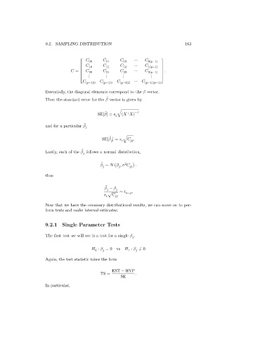
Essentially, the diagonal elements correspond to the vector.
̂
Then the standard error for the vector is given by

̂
⊤
SE[ ] = √ ( ) −1
and for a particular ̂

̂
SE[ ] = √ .

̂
Lastly, each of the follows a normal distribution,

̂
2
∼ ( , ) .

thus
̂
−

√ ∼ − .

Now that we have the necessary distributional results, we can move on to per-
form tests and make interval estimates.

9.2.1 Single Parameter Tests

The first test we will see is a test for a single .

∶ = 0 vs ∶ ≠ 0
1

0

Again, the test statistic takes the form
EST − HYP
TS = .
SE
In particular,