Page 243 - Applied Statistics with R

12.3. ONE-WAY ANOVA 243

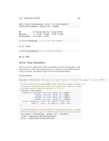
good = data.frame(response, group = as.factor(group))
summary(aov(response ~ group, data = good))

## Df Sum Sq Mean Sq F value Pr(>F)
## group 2 0.232 0.1158 0.096 0.909
## Residuals 12 14.484 1.2070

is.factor(bad$group) # 1, 2, and 3 are numbers.

## [1] FALSE

is.factor(good$group) # 1, 2, and 3 are labels.

## [1] TRUE

12.3.2 Some Simulation

Here we verify the distribution of the test statistic under the null hypothesis. We
simulate from a null model (equal variance) to obtain an empirical distribution
of the statistic. We add the curve for the expected distribution.
library(broom)

sim_anova = function(n = 10, mu_a = 0, mu_b = 0, mu_c = 0, mu_d = 0, sigma = 1, stat = TRUE) {
# create data from one-way ANOVA model with four groups of equal size
# response simulated from normal with group mean, shared variance
# group variable indicates group A, B, C or D
sim_data = data.frame(
response = c(rnorm(n = n, mean = mu_a, sd = sigma),
rnorm(n = n, mean = mu_b, sd = sigma),
rnorm(n = n, mean = mu_c, sd = sigma),
rnorm(n = n, mean = mu_d, sd = sigma)),
group = c(rep("A", times = n), rep("B", times = n),
rep("C", times = n), rep("D", times = n))
)

# obtain F-statistic and p-value for testing difference of means
# use lm instead of aov for better result formatting with glance
aov_results = lm(response ~ group, data = sim_data)
f_stat = glance(aov_results)$statistic
p_val = glance(aov_results)$p.value