Page 272 - Applied Statistics with R

272 CHAPTER 13. MODEL DIAGNOSTICS

Lastly, for fit_3 we again see a large p-value, so we do not reject the null of
homoscedasticity, which matches our findings with a fitted versus residuals plot.

13.2.3 Histograms

We have a number of tools for assessing the normality assumption. The most
obvious would be to make a histogram of the residuals. If it appears roughly
normal, then we’ll believe the errors could truly be normal.

par(mfrow = c(1, 3))
hist(resid(fit_1),
xlab = "Residuals",
main = "Histogram of Residuals, fit_1",
col = "darkorange",
border = "dodgerblue",
breaks = 20)
hist(resid(fit_2),
xlab = "Residuals",
main = "Histogram of Residuals, fit_2",
col = "darkorange",
border = "dodgerblue",
breaks = 20)
hist(resid(fit_3),
xlab = "Residuals",
main = "Histogram of Residuals, fit_3",
col = "darkorange",
border = "dodgerblue",
breaks = 20)

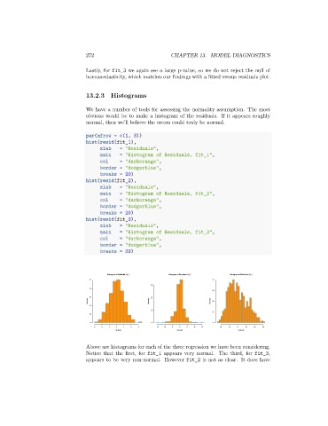
Histogram of Residuals, fit_1 Histogram of Residuals, fit_2 Histogram of Residuals, fit_3
100 40
150
80
30
60 100
Frequency Frequency Frequency 20
40
50
10
20
0 0 0
-3 -2 -1 0 1 2 3 -15 -10 -5 0 5 10 15 -20 -10 0 10 20 30
Residuals Residuals Residuals

Above are histograms for each of the three regression we have been considering.
Notice that the first, for fit_1 appears very normal. The third, for fit_3,
appears to be very non-normal. However fit_2 is not as clear. It does have