Page 275 - Applied Statistics with R

13.2. CHECKING ASSUMPTIONS 275

Normal Q-Q Plot Normal Q-Q Plot
2 2

1 1
Sample Quantiles 0 -1 Sample Quantiles 0 -1

-2 -2

-3 -3
-2 -1 0 1 2 -2 -1 0 1 2
Theoretical Quantiles Theoretical Quantiles

To get a better idea of what “close to the line” means, we perform a number of
simulations, and create Q-Q plots.

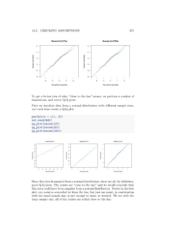
First we simulate data from a normal distribution with different sample sizes,
and each time create a Q-Q plot.

par(mfrow = c(1, 3))
set.seed(420)
qq_plot(rnorm(10))
qq_plot(rnorm(25))
qq_plot(rnorm(100))

Normal Q-Q Plot Normal Q-Q Plot Normal Q-Q Plot
2.0 2
0.5
1.5
0.0 1
-0.5 1.0
Sample Quantiles -1.0 -1.5 Sample Quantiles 0.5 0.0 Sample Quantiles 0
-2.0 -0.5 -1
-2
-2.5 -1.0
-3.0 -3
-1.5 -1.0 -0.5 0.0 0.5 1.0 1.5 -2 -1 0 1 2 -2 -1 0 1 2
Theoretical Quantiles Theoretical Quantiles Theoretical Quantiles

Since this data is sampled from a normal distribution, these are all, by definition,
good Q-Q plots. The points are “close to the line” and we would conclude that
this data could have been sampled from a normal distribution. Notice in the first
plot, one point is somewhat far from the line, but just one point, in combination
with the small sample size, is not enough to make us worried. We see with the
large sample size, all of the points are rather close to the line.