Page 277 - Applied Statistics with R

13.2. CHECKING ASSUMPTIONS 277

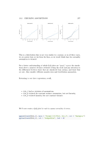
Normal Q-Q Plot Normal Q-Q Plot Normal Q-Q Plot
2.0 7
4
6
1.5
5
3
Sample Quantiles 1.0 Sample Quantiles 4 3 Sample Quantiles 2
0.5 2 1
1
0.0 0 0
-1.5 -1.0 -0.5 0.0 0.5 1.0 1.5 -2 -1 0 1 2 -2 -1 0 1 2
Theoretical Quantiles Theoretical Quantiles Theoretical Quantiles

This is a distribution that is not very similar to a normal, so in all three cases,
we see points that are far from the lines, so we would think that the normality
assumption is violated.

For a better understanding of which Q-Q plots are “good,” repeat the simula-
tions above a number of times (without setting the seed) and pay attention to
the differences between those that are simulated from normal, and those that
are not. Also consider different samples sizes and distribution parameters.

Returning to our three regressions, recall,

• fit_1 had no violation of assumptions,
• fit_2 violated the constant variance assumption, but not linearity,
• fit_3 violated linearity, but not constant variance.

We’ll now create a Q-Q plot for each to assess normality of errors.

qqnorm(resid(fit_1), main = "Normal Q-Q Plot, fit_1", col = "darkgrey")
qqline(resid(fit_1), col = "dodgerblue", lwd = 2)