Page 329 - Applied Statistics with R

14.2. PREDICTOR TRANSFORMATION 329

300

100
y

-100

-300

0 2 4 6 8 10

x

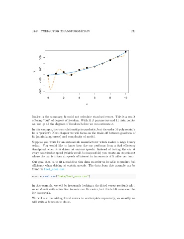
Notice in the summary, R could not calculate standard errors. This is a result
of being “out” of degrees of freedom. With 11 parameters and 11 data points,
we use up all the degrees of freedom before we can estimate .
In this example, the true relationship is quadratic, but the order 10 polynomial’s
fit is “perfect”. Next chapter we will focus on the trade-off between goodness of
fit (minimizing errors) and complexity of model.
Suppose you work for an automobile manufacturer which makes a large luxury
sedan. You would like to know how the car performs from a fuel efficiency
standpoint when it is driven at various speeds. Instead of testing the car at
every conceivable speed (which would be impossible) you create an experiment
where the car is driven at speeds of interest in increments of 5 miles per hour.
Our goal then, is to fit a model to this data in order to be able to predict fuel
efficiency when driving at certain speeds. The data from this example can be
found in fuel_econ.csv.

econ = read.csv("data/fuel_econ.csv")

In this example, we will be frequently looking a the fitted versus residuals plot,
so we should write a function to make our life easier, but this is left as an exercise
for homework.

We will also be adding fitted curves to scatterplots repeatedly, so smartly we
will write a function to do so.