Page 330 - Applied Statistics with R

330 CHAPTER 14. TRANSFORMATIONS

plot_econ_curve = function(model) {
plot(mpg ~ mph, data = econ, xlab = "Speed (Miles per Hour)",
ylab = "Fuel Efficiency (Miles per Gallon)", col = "dodgerblue",
pch = 20, cex = 2)
xplot = seq(10, 75, by = 0.1)
lines(xplot, predict(model, newdata = data.frame(mph = xplot)),
col = "darkorange", lwd = 2, lty = 1)
}

So now we first fit a simple linear regression to this data.

fit1 = lm(mpg ~ mph, data = econ)

par(mfrow = c(1, 2))
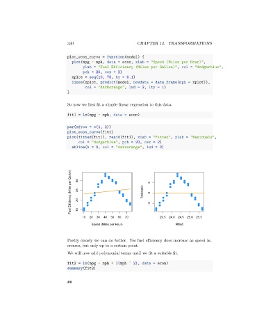
plot_econ_curve(fit1)
plot(fitted(fit1), resid(fit1), xlab = "Fitted", ylab = "Residuals",
col = "dodgerblue", pch = 20, cex = 2)
abline(h = 0, col = "darkorange", lwd = 2)

Fuel Efficiency (Miles per Gallon) 30 25 20 Residuals 5 0 -5

15
10 20 30 40 50 60 70 23.5 24.0 24.5 25.0 25.5
Speed (Miles per Hour) Fitted

Pretty clearly we can do better. Yes fuel efficiency does increase as speed in-
creases, but only up to a certain point.
We will now add polynomial terms until we fit a suitable fit.

fit2 = lm(mpg ~ mph + I(mph ^ 2), data = econ)
summary(fit2)

##