Page 331 - Applied Statistics with R

14.2. PREDICTOR TRANSFORMATION 331

## Call:
## lm(formula = mpg ~ mph + I(mph^2), data = econ)
##
## Residuals:
## Min 1Q Median 3Q Max
## -2.8411 -0.9694 0.0017 1.0181 3.3900
##
## Coefficients:
## Estimate Std. Error t value Pr(>|t|)
## (Intercept) 2.4444505 1.4241091 1.716 0.0984 .
## mph 1.2716937 0.0757321 16.792 3.99e-15 ***
## I(mph^2) -0.0145014 0.0008719 -16.633 4.97e-15 ***
## ---
## Signif. codes: 0 '***' 0.001 '**' 0.01 '*' 0.05 '.' 0.1 ' ' 1
##
## Residual standard error: 1.663 on 25 degrees of freedom
## Multiple R-squared: 0.9188, Adjusted R-squared: 0.9123
## F-statistic: 141.5 on 2 and 25 DF, p-value: 2.338e-14

par(mfrow = c(1, 2))
plot_econ_curve(fit2)
plot(fitted(fit2), resid(fit2), xlab = "Fitted", ylab = "Residuals",
col = "dodgerblue", pch = 20, cex = 2)
abline(h = 0, col = "darkorange", lwd = 2)

Fuel Efficiency (Miles per Gallon) 30 25 20 Residuals 3 2 1 0 -1

15

10 20 30 40 50 60 70 -2 -3 15 20 25 30
Speed (Miles per Hour) Fitted

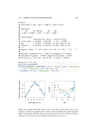
While this model clearly fits much better, and the second order term is sig-
nificant, we still see a pattern in the fitted versus residuals plot which suggests
higher order terms will help. Also, we would expect the curve to flatten as speed
increases or decreases, not go sharply downward as we see here.