Page 176 - Python Data Science Handbook

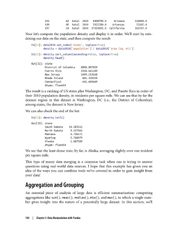
101 AZ total 2010 6408790.0 Arizona 114006.0
189 AR total 2010 2922280.0 Arkansas 53182.0
197 CA total 2010 37333601.0 California 163707.0
Now let’s compute the population density and display it in order. We’ll start by rein‐
dexing our data on the state, and then compute the result:
In[31]: data2010.set_index('state', inplace=True)
density = data2010['population'] / data2010['area (sq. mi)']
In[32]: density.sort_values(ascending=False, inplace=True)
density.head()
Out[32]: state
District of Columbia 8898.897059
Puerto Rico 1058.665149
New Jersey 1009.253268
Rhode Island 681.339159
Connecticut 645.600649
dtype: float64
The result is a ranking of US states plus Washington, DC, and Puerto Rico in order of
their 2010 population density, in residents per square mile. We can see that by far the
densest region in this dataset is Washington, DC (i.e., the District of Columbia);
among states, the densest is New Jersey.
We can also check the end of the list:

In[33]: density.tail()
Out[33]: state
South Dakota 10.583512
North Dakota 9.537565
Montana 6.736171
Wyoming 5.768079
Alaska 1.087509
dtype: float64
We see that the least dense state, by far, is Alaska, averaging slightly over one resident
per square mile.
This type of messy data merging is a common task when one is trying to answer
questions using real-world data sources. I hope that this example has given you an
idea of the ways you can combine tools we’ve covered in order to gain insight from
your data!

Aggregation and Grouping

An essential piece of analysis of large data is efficient summarization: computing
aggregations like sum(), mean(), median(), min(), and max(), in which a single num‐
ber gives insight into the nature of a potentially large dataset. In this section, we’ll

158 | Chapter 3: Data Manipulation with Pandas