Page 291 - Python Data Science Handbook

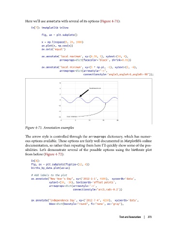
Here we’ll use annotate with several of its options (Figure 4-71):
In[7]: %matplotlib inline

fig, ax = plt.subplots()
x = np.linspace(0, 20, 1000)
ax.plot(x, np.cos(x))
ax.axis('equal')

ax.annotate('local maximum', xy=(6.28, 1), xytext=(10, 4),
arrowprops=dict(facecolor='black', shrink=0.05))
ax.annotate('local minimum', xy=(5 * np.pi, -1), xytext=(2, -6),
arrowprops=dict(arrowstyle="->",
connectionstyle="angle3,angleA=0,angleB=-90"));

Figure 4-71. Annotation examples

The arrow style is controlled through the arrowprops dictionary, which has numer‐
ous options available. These options are fairly well documented in Matplotlib’s online
documentation, so rather than repeating them here I’ll quickly show some of the pos‐
sibilities. Let’s demonstrate several of the possible options using the birthrate plot
from before (Figure 4-72):
In[8]:
fig, ax = plt.subplots(figsize=(12, 4))
births_by_date.plot(ax=ax)

# Add labels to the plot
ax.annotate("New Year's Day", xy=('2012-1-1', 4100), xycoords='data',
xytext=(50, -30), textcoords='offset points',
arrowprops=dict(arrowstyle="->",
connectionstyle="arc3,rad=-0.2"))

ax.annotate("Independence Day", xy=('2012-7-4', 4250), xycoords='data',
bbox=dict(boxstyle="round", fc="none", ec="gray"),

Text and Annotation | 273