Page 422 - Python Data Science Handbook

failed to take into account (e.g., perhaps people ride less at both high and low temper‐
atures). Nevertheless, our rough approximation is enough to give us some insights,
and we can take a look at the coefficients of the linear model to estimate how much
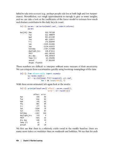
each feature contributes to the daily bicycle count:

In[24]: params = pd.Series(model.coef_, index=X.columns)
params
Out[24]: Mon 503.797330
Tue 612.088879
Wed 591.611292
Thu 481.250377
Fri 176.838999
Sat -1104.321406
Sun -1134.610322
holiday -1187.212688
daylight_hrs 128.873251
PRCP -665.185105
dry day 546.185613
Temp (C) 65.194390
annual 27.865349
dtype: float64
These numbers are difficult to interpret without some measure of their uncertainty.
We can compute these uncertainties quickly using bootstrap resamplings of the data:

In[25]: from sklearn.utils import resample
np.random.seed(1)
err = np.std([model.fit(*resample(X, y)).coef_
for i in range(1000)], 0)
With these errors estimated, let’s again look at the results:

In[26]: print(pd.DataFrame({'effect': params.round(0),
'error': err.round(0)}))
effect error
Mon 504 85
Tue 612 82
Wed 592 82
Thu 481 85
Fri 177 81
Sat -1104 79
Sun -1135 82
holiday -1187 164
daylight_hrs 129 9
PRCP -665 62
dry day 546 33
Temp (C) 65 4
annual 28 18
We first see that there is a relatively stable trend in the weekly baseline: there are
many more riders on weekdays than on weekends and holidays. We see that for each

404 | Chapter 5: Machine Learning