Page 421 - Python Data Science Handbook

2012-10-07 2142 0 0 0 0 0 0 1 0 11.045208
PRCP Temp (C) dry day annual
Date
2012-10-03 0 13.35 1 0.000000
2012-10-04 0 13.60 1 0.002740
2012-10-05 0 15.30 1 0.005479
2012-10-06 0 15.85 1 0.008219
2012-10-07 0 15.85 1 0.010959
With this in place, we can choose the columns to use, and fit a linear regression
model to our data. We will set fit_intercept = False, because the daily flags essen‐
tially operate as their own day-specific intercepts:

In[22]:
column_names = ['Mon', 'Tue', 'Wed', 'Thu', 'Fri', 'Sat', 'Sun', 'holiday',
'daylight_hrs', 'PRCP', 'dry day', 'Temp (C)', 'annual']
X = daily[column_names]
y = daily['Total']
model = LinearRegression(fit_intercept=False)
model.fit(X, y)
daily['predicted'] = model.predict(X)
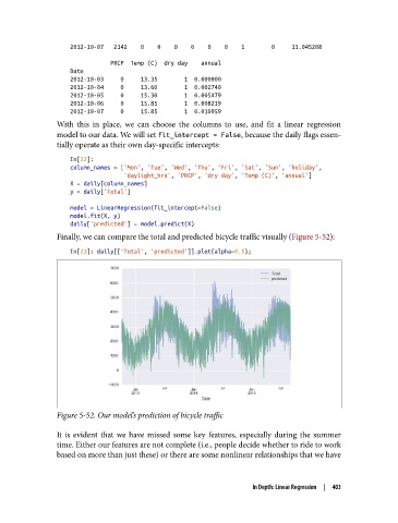
Finally, we can compare the total and predicted bicycle traffic visually (Figure 5-52):

In[23]: daily[['Total', 'predicted']].plot(alpha=0.5);

Figure 5-52. Our model’s prediction of bicycle tra‘c

It is evident that we have missed some key features, especially during the summer
time. Either our features are not complete (i.e., people decide whether to ride to work
based on more than just these) or there are some nonlinear relationships that we have

In Depth: Linear Regression | 403