Page 476 - Python Data Science Handbook

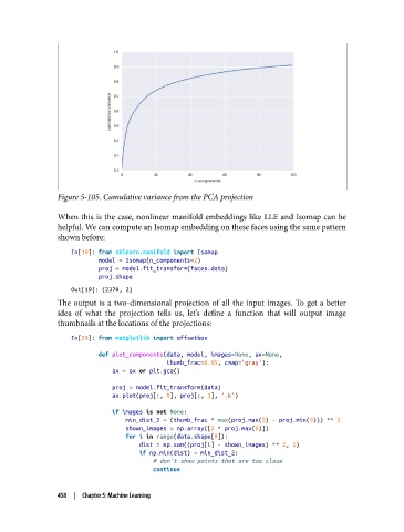
Figure 5-105. Cumulative variance from the PCA projection

When this is the case, nonlinear manifold embeddings like LLE and Isomap can be
helpful. We can compute an Isomap embedding on these faces using the same pattern
shown before:

In[19]: from sklearn.manifold import Isomap
model = Isomap(n_components=2)
proj = model.fit_transform(faces.data)
proj.shape
Out[19]: (2370, 2)
The output is a two-dimensional projection of all the input images. To get a better
idea of what the projection tells us, let’s define a function that will output image
thumbnails at the locations of the projections:

In[20]: from matplotlib import offsetbox
def plot_components(data, model, images=None, ax=None,
thumb_frac=0.05, cmap='gray'):
ax = ax or plt.gca()

proj = model.fit_transform(data)
ax.plot(proj[:, 0], proj[:, 1], '.k')

if images is not None:
min_dist_2 = (thumb_frac * max(proj.max(0) - proj.min(0))) ** 2
shown_images = np.array([2 * proj.max(0)])
for i in range(data.shape[0]):
dist = np.sum((proj[i] - shown_images) ** 2, 1)
if np.min(dist) < min_dist_2:
# don't show points that are too close
continue

458 | Chapter 5: Machine Learning