Page 475 - Python Data Science Handbook

We have 2,370 images, each with 2,914 pixels. In other words, the images can be
thought of as data points in a 2,914-dimensional space!
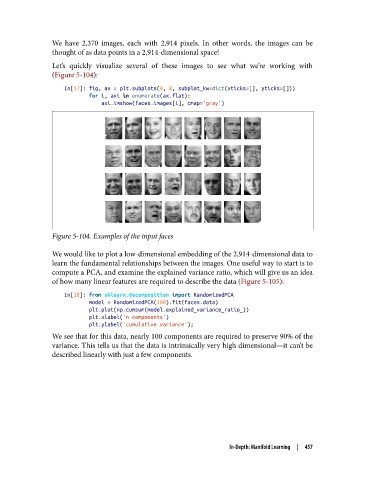
Let’s quickly visualize several of these images to see what we’re working with
(Figure 5-104):

In[17]: fig, ax = plt.subplots(4, 8, subplot_kw=dict(xticks=[], yticks=[]))
for i, axi in enumerate(ax.flat):
axi.imshow(faces.images[i], cmap='gray')

Figure 5-104. Examples of the input faces

We would like to plot a low-dimensional embedding of the 2,914-dimensional data to
learn the fundamental relationships between the images. One useful way to start is to
compute a PCA, and examine the explained variance ratio, which will give us an idea
of how many linear features are required to describe the data (Figure 5-105):
In[18]: from sklearn.decomposition import RandomizedPCA
model = RandomizedPCA(100).fit(faces.data)
plt.plot(np.cumsum(model.explained_variance_ratio_))
plt.xlabel('n components')
plt.ylabel('cumulative variance');
We see that for this data, nearly 100 components are required to preserve 90% of the
variance. This tells us that the data is intrinsically very high dimensional—it can’t be
described linearly with just a few components.

In-Depth: Manifold Learning | 457