Page 490 - Python Data Science Handbook

In[15]: from sklearn.metrics import accuracy_score
accuracy_score(digits.target, labels)
Out[15]: 0.79354479688369506
With just a simple k-means algorithm, we discovered the correct grouping for 80% of
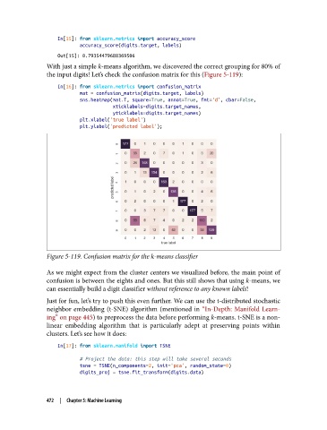
the input digits! Let’s check the confusion matrix for this (Figure 5-119):

In[16]: from sklearn.metrics import confusion_matrix
mat = confusion_matrix(digits.target, labels)
sns.heatmap(mat.T, square=True, annot=True, fmt='d', cbar=False,
xticklabels=digits.target_names,
yticklabels=digits.target_names)
plt.xlabel('true label')
plt.ylabel('predicted label');

Figure 5-119. Confusion matrix for the k-means classifier

As we might expect from the cluster centers we visualized before, the main point of
confusion is between the eights and ones. But this still shows that using k-means, we
can essentially build a digit classifier without reference to any known labels!
Just for fun, let’s try to push this even further. We can use the t-distributed stochastic
neighbor embedding (t-SNE) algorithm (mentioned in “In-Depth: Manifold Learn‐
ing” on page 445) to preprocess the data before performing k-means. t-SNE is a non‐
linear embedding algorithm that is particularly adept at preserving points within
clusters. Let’s see how it does:

In[17]: from sklearn.manifold import TSNE
# Project the data: this step will take several seconds
tsne = TSNE(n_components=2, init='pca', random_state=0)
digits_proj = tsne.fit_transform(digits.data)

472 | Chapter 5: Machine Learning