Page 88 - Class-11-Physics-Part-1_Neat

74 PHYSICS

∆t , respectively. The direction of the average
3
velocity v is shown in figures (a), (b) and (c) for
three decreasing values of ∆t, i.e. ∆t ,∆t , and ∆t ,
3
2
1
→ →
(∆t > ∆t > ∆t ). As ∆t →→ →→ → 0, ∆r → → → 0
1 2 3
and is along the tangent to the path [Fig. 4.13(d)].
Therefore, the direction of velocity at any point
on the path of an object is tangential to the
path at that point and is in the direction of
motion.
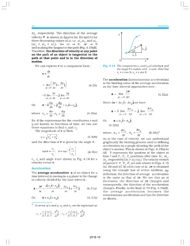
We can express v in a component form : Fig. 4.14 The components v and v y of velocity v and
x

the angle θ it makes with x-axis. Note that
d r
v = v = v cos θ, v = v sin θ.
y
x
dt
The acceleration (instantaneous acceleration)
 x∆ ∆ y  is the limiting value of the average acceleration
= lim  i +  j (4.29)
t ∆ →0  t∆ t ∆  as the time interval approaches zero :
∆ v
∆ x ∆ y

= i lim + j lim a = lim ∆ (4.32a)
t ∆ → ∆0 t t ∆ → ∆0 t ∆ t → 0 t
dx dy Since ∆v = ∆v i + ∆v j ,we have
x
y

Or, v = i + j = v x i + v y j.
dt dt ∆ v ∆ v

d x d y a = i lim x + j lim y
where v = , v = (4.30a) ∆ ∆
x y ∆ t → 0 t ∆ t → 0 t
t d t d
So, if the expressions for the coordinates x and Or, a = a i + a j
x y
y are known as functions of time, we can use (4.32b)
these equations to find v and v .
x y d v
The magnitude of v is then d v x y
where, a = , a = (4.32c)*
x y
t d
t d
2
v = v + v y 2 (4.30b) As in the case of velocity, we can understand
x
and the direction of v is given by the angle θ : graphically the limiting process used in defining
acceleration on a graph showing the path of the
 
v y v y object’s motion. This is shown in Figs. 4.15(a) to
tanθ = , θ = tan − 1    (4.30c)
v   v  (d). P represents the position of the object at
x x
time t and P , P , P positions after time ∆t , ∆t ,
2
1
2
1
3
v , v and angle θ are shown in Fig. 4.14 for a ∆t , respectively (∆t > ∆t >∆t ). The velocity vectors
x y 3 1 2 3
velocity vector v. at points P, P , P , P are also shown in Figs. 4.15
1 2 3
(a), (b) and (c). In each case of ∆t, ∆v is obtained
Acceleration
using the triangle law of vector addition. By
The average acceleration a of an object for a
definition, the direction of average acceleration
time interval ∆t moving in x-y plane is the change
is the same as that of ∆v. We see that as ∆t
in velocity divided by the time interval :
decreases, the direction of ∆v changes and
∆ v ( ∆ v x i + v y ) j ∆v ∆v consequently, the direction of the acceleration
a = = = x i + y j (4.31a) changes. Finally, in the limit ∆t g0 [Fig. 4.15(d)],
∆t ∆t ∆t ∆t the average acceleration becomes the
instantaneous acceleration and has the direction
Or, a = a i + a j. (4.31b)
x y as shown.
* In terms of x and y, a and a can be expressed as
x y

2018-19