Page 163 - Python Data Science Handbook

The result is a multiply indexed DataFrame, and we can use the tools discussed in
“Hierarchical Indexing” on page 128 to transform this data into the representation
we’re interested in.

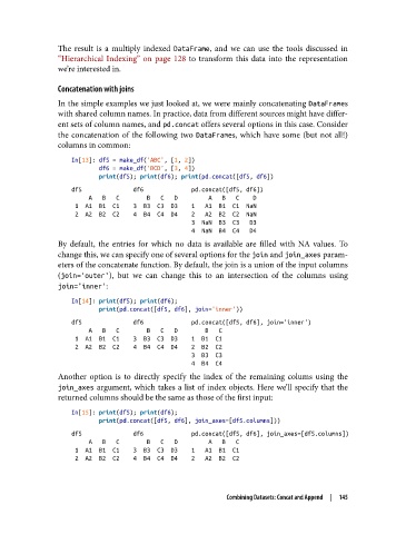
Concatenation with joins
In the simple examples we just looked at, we were mainly concatenating DataFrames
with shared column names. In practice, data from different sources might have differ‐
ent sets of column names, and pd.concat offers several options in this case. Consider
the concatenation of the following two DataFrames, which have some (but not all!)
columns in common:
In[13]: df5 = make_df('ABC', [1, 2])
df6 = make_df('BCD', [3, 4])
print(df5); print(df6); print(pd.concat([df5, df6])
df5 df6 pd.concat([df5, df6])
A B C B C D A B C D
1 A1 B1 C1 3 B3 C3 D3 1 A1 B1 C1 NaN
2 A2 B2 C2 4 B4 C4 D4 2 A2 B2 C2 NaN
3 NaN B3 C3 D3
4 NaN B4 C4 D4
By default, the entries for which no data is available are filled with NA values. To
change this, we can specify one of several options for the join and join_axes param‐
eters of the concatenate function. By default, the join is a union of the input columns
(join='outer'), but we can change this to an intersection of the columns using
join='inner':

In[14]: print(df5); print(df6);
print(pd.concat([df5, df6], join='inner'))
df5 df6 pd.concat([df5, df6], join='inner')
A B C B C D B C
1 A1 B1 C1 3 B3 C3 D3 1 B1 C1
2 A2 B2 C2 4 B4 C4 D4 2 B2 C2
3 B3 C3
4 B4 C4
Another option is to directly specify the index of the remaining colums using the
join_axes argument, which takes a list of index objects. Here we’ll specify that the
returned columns should be the same as those of the first input:
In[15]: print(df5); print(df6);
print(pd.concat([df5, df6], join_axes=[df5.columns]))

df5 df6 pd.concat([df5, df6], join_axes=[df5.columns])
A B C B C D A B C
1 A1 B1 C1 3 B3 C3 D3 1 A1 B1 C1
2 A2 B2 C2 4 B4 C4 D4 2 A2 B2 C2

Combining Datasets: Concat and Append | 145