Page 356 - Python Data Science Handbook

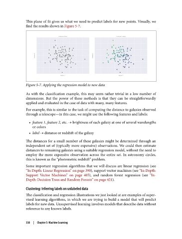
This plane of fit gives us what we need to predict labels for new points. Visually, we
find the results shown in Figure 5-7.

Figure 5-7. Applying the regression model to new data

As with the classification example, this may seem rather trivial in a low number of
dimensions. But the power of these methods is that they can be straightforwardly
applied and evaluated in the case of data with many, many features.
For example, this is similar to the task of computing the distance to galaxies observed
through a telescope—in this case, we might use the following features and labels:

• feature 1, feature 2, etc. brightness of each galaxy at one of several wavelengths
or colors
• label distance or redshift of the galaxy

The distances for a small number of these galaxies might be determined through an
independent set of (typically more expensive) observations. We could then estimate
distances to remaining galaxies using a suitable regression model, without the need to
employ the more expensive observation across the entire set. In astronomy circles,
this is known as the “photometric redshift” problem.
Some important regression algorithms that we will discuss are linear regression (see
“In Depth: Linear Regression” on page 390), support vector machines (see “In-Depth:
Support Vector Machines” on page 405), and random forest regression (see “In-
Depth: Decision Trees and Random Forests” on page 421).

Clustering: Inferring labels on unlabeled data
The classification and regression illustrations we just looked at are examples of super‐
vised learning algorithms, in which we are trying to build a model that will predict
labels for new data. Unsupervised learning involves models that describe data without
reference to any known labels.

338 | Chapter 5: Machine Learning