Page 385 - Python Data Science Handbook

In[10]: from sklearn.preprocessing import PolynomialFeatures
from sklearn.linear_model import LinearRegression
from sklearn.pipeline import make_pipeline

def PolynomialRegression(degree=2, **kwargs):
return make_pipeline(PolynomialFeatures(degree),
LinearRegression(**kwargs))
Now let’s create some data to which we will fit our model:

In[11]: import numpy as np
def make_data(N, err=1.0, rseed=1):
# randomly sample the data
rng = np.random.RandomState(rseed)
X = rng.rand(N, 1) ** 2
y = 10 - 1. / (X.ravel() + 0.1)
if err > 0:
y += err * rng.randn(N)
return X, y

X, y = make_data(40)
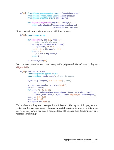
We can now visualize our data, along with polynomial fits of several degrees
(Figure 5-27):

In[12]: %matplotlib inline
import matplotlib.pyplot as plt
import seaborn; seaborn.set() # plot formatting

X_test = np.linspace(-0.1, 1.1, 500)[:, None]
plt.scatter(X.ravel(), y, color='black')
axis = plt.axis()
for degree in [1, 3, 5]:
y_test = PolynomialRegression(degree).fit(X, y).predict(X_test)
plt.plot(X_test.ravel(), y_test, label='degree={0}'.format(degree))
plt.xlim(-0.1, 1.0)
plt.ylim(-2, 12)
plt.legend(loc='best');
The knob controlling model complexity in this case is the degree of the polynomial,
which can be any non-negative integer. A useful question to answer is this: what
degree of polynomial provides a suitable trade-off between bias (underfitting) and
variance (overfitting)?

Hyperparameters and Model Validation | 367