Page 390 - Python Data Science Handbook

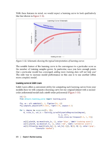
With these features in mind, we would expect a learning curve to look qualitatively
like that shown in Figure 5-32.

Figure 5-32. Schematic showing the typical interpretation of learning curves

The notable feature of the learning curve is the convergence to a particular score as
the number of training samples grows. In particular, once you have enough points
that a particular model has converged, adding more training data will not help you!
The only way to increase model performance in this case is to use another (often
more complex) model.

Learning curves in Scikit-Learn
Scikit-Learn offers a convenient utility for computing such learning curves from your
models; here we will compute a learning curve for our original dataset with a second-
order polynomial model and a ninth-order polynomial (Figure 5-33):

In[17]:
from sklearn.learning_curve import learning_curve

fig, ax = plt.subplots(1, 2, figsize=(16, 6))
fig.subplots_adjust(left=0.0625, right=0.95, wspace=0.1)

for i, degree in enumerate([2, 9]):
N, train_lc, val_lc = learning_curve(PolynomialRegression(degree),
X, y, cv=7,
train_sizes=np.linspace(0.3, 1, 25))

ax[i].plot(N, np.mean(train_lc, 1), color='blue', label='training score')
ax[i].plot(N, np.mean(val_lc, 1), color='red', label='validation score')
ax[i].hlines(np.mean([train_lc[-1], val_lc[-1]]), N[0], N[-1], color='gray',
linestyle='dashed')

372 | Chapter 5: Machine Learning