Page 386 - Python Data Science Handbook

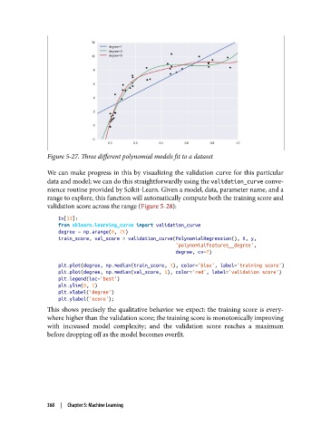
Figure 5-27. Three different polynomial models fit to a dataset

We can make progress in this by visualizing the validation curve for this particular
data and model; we can do this straightforwardly using the validation_curve conve‐
nience routine provided by Scikit-Learn. Given a model, data, parameter name, and a
range to explore, this function will automatically compute both the training score and
validation score across the range (Figure 5-28):

In[13]:
from sklearn.learning_curve import validation_curve
degree = np.arange(0, 21)
train_score, val_score = validation_curve(PolynomialRegression(), X, y,
'polynomialfeatures__degree',
degree, cv=7)

plt.plot(degree, np.median(train_score, 1), color='blue', label='training score')
plt.plot(degree, np.median(val_score, 1), color='red', label='validation score')
plt.legend(loc='best')
plt.ylim(0, 1)
plt.xlabel('degree')
plt.ylabel('score');
This shows precisely the qualitative behavior we expect: the training score is every‐
where higher than the validation score; the training score is monotonically improving
with increased model complexity; and the validation score reaches a maximum
before dropping off as the model becomes overfit.

368 | Chapter 5: Machine Learning