Page 388 - Python Data Science Handbook

Notice that finding this optimal model did not actually require us to compute the
training score, but examining the relationship between the training score and valida‐
tion score can give us useful insight into the performance of the model.
Learning Curves

One important aspect of model complexity is that the optimal model will generally
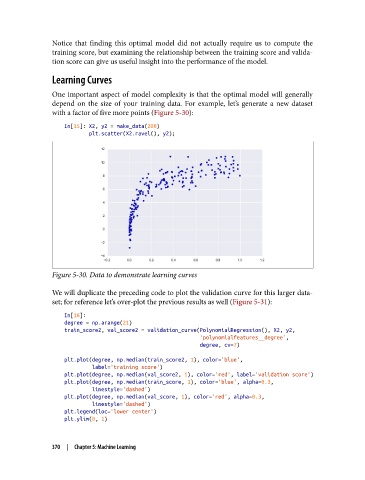
depend on the size of your training data. For example, let’s generate a new dataset
with a factor of five more points (Figure 5-30):

In[15]: X2, y2 = make_data(200)
plt.scatter(X2.ravel(), y2);

Figure 5-30. Data to demonstrate learning curves

We will duplicate the preceding code to plot the validation curve for this larger data‐
set; for reference let’s over-plot the previous results as well (Figure 5-31):

In[16]:
degree = np.arange(21)
train_score2, val_score2 = validation_curve(PolynomialRegression(), X2, y2,
'polynomialfeatures__degree',
degree, cv=7)
plt.plot(degree, np.median(train_score2, 1), color='blue',
label='training score')
plt.plot(degree, np.median(val_score2, 1), color='red', label='validation score')
plt.plot(degree, np.median(train_score, 1), color='blue', alpha=0.3,
linestyle='dashed')
plt.plot(degree, np.median(val_score, 1), color='red', alpha=0.3,
linestyle='dashed')
plt.legend(loc='lower center')
plt.ylim(0, 1)

370 | Chapter 5: Machine Learning