Page 391 - Python Data Science Handbook

ax[i].set_ylim(0, 1)
ax[i].set_xlim(N[0], N[-1])
ax[i].set_xlabel('training size')
ax[i].set_ylabel('score')
ax[i].set_title('degree = {0}'.format(degree), size=14)
ax[i].legend(loc='best')

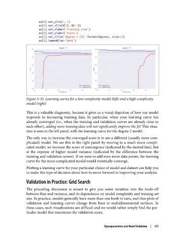
Figure 5-33. Learning curves for a low-complexity model (left) and a high-complexity
model (right)

This is a valuable diagnostic, because it gives us a visual depiction of how our model
responds to increasing training data. In particular, when your learning curve has
already converged (i.e., when the training and validation curves are already close to
each other), adding more training data will not significantly improve the fit! This situa‐
tion is seen in the left panel, with the learning curve for the degree-2 model.
The only way to increase the converged score is to use a different (usually more com‐
plicated) model. We see this in the right panel: by moving to a much more compli‐
cated model, we increase the score of convergence (indicated by the dashed line), but
at the expense of higher model variance (indicated by the difference between the
training and validation scores). If we were to add even more data points, the learning
curve for the more complicated model would eventually converge.
Plotting a learning curve for your particular choice of model and dataset can help you
to make this type of decision about how to move forward in improving your analysis.

Validation in Practice: Grid Search

The preceding discussion is meant to give you some intuition into the trade-off
between bias and variance, and its dependence on model complexity and training set
size. In practice, models generally have more than one knob to turn, and thus plots of
validation and learning curves change from lines to multidimensional surfaces. In
these cases, such visualizations are difficult and we would rather simply find the par‐
ticular model that maximizes the validation score.

Hyperparameters and Model Validation | 373