Page 396 - Python Data Science Handbook

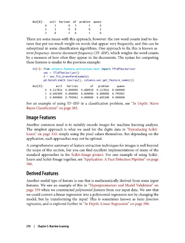
Out[8]: evil horizon of problem queen
0 1 0 1 1 0
1 1 0 0 0 1
2 0 1 0 1 0
There are some issues with this approach, however: the raw word counts lead to fea‐
tures that put too much weight on words that appear very frequently, and this can be
suboptimal in some classification algorithms. One approach to fix this is known as
term frequency–inverse document frequency (TF–IDF), which weights the word counts
by a measure of how often they appear in the documents. The syntax for computing
these features is similar to the previous example:

In[9]: from sklearn.feature_extraction.text import TfidfVectorizer
vec = TfidfVectorizer()
X = vec.fit_transform(sample)
pd.DataFrame(X.toarray(), columns=vec.get_feature_names())
Out[9]: evil horizon of problem queen
0 0.517856 0.000000 0.680919 0.517856 0.000000
1 0.605349 0.000000 0.000000 0.000000 0.795961
2 0.000000 0.795961 0.000000 0.605349 0.000000
For an example of using TF–IDF in a classification problem, see “In Depth: Naive
Bayes Classification” on page 382.

Image Features

Another common need is to suitably encode images for machine learning analysis.
The simplest approach is what we used for the digits data in “Introducing Scikit-
Learn” on page 343: simply using the pixel values themselves. But depending on the
application, such approaches may not be optimal.

A comprehensive summary of feature extraction techniques for images is well beyond
the scope of this section, but you can find excellent implementations of many of the
standard approaches in the Scikit-Image project. For one example of using Scikit-
Learn and Scikit-Image together, see “Application: A Face Detection Pipeline” on page
506.

Derived Features

Another useful type of feature is one that is mathematically derived from some input
features. We saw an example of this in “Hyperparameters and Model Validation” on
page 359 when we constructed polynomial features from our input data. We saw that
we could convert a linear regression into a polynomial regression not by changing the
model, but by transforming the input! This is sometimes known as basis function
regression, and is explored further in “In Depth: Linear Regression” on page 390.

378 | Chapter 5: Machine Learning