Page 429 - Python Data Science Handbook

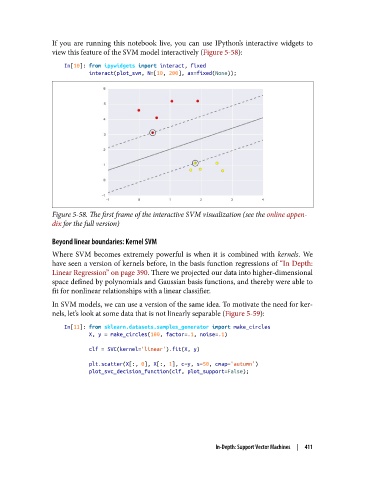
If you are running this notebook live, you can use IPython’s interactive widgets to
view this feature of the SVM model interactively (Figure 5-58):

In[10]: from ipywidgets import interact, fixed
interact(plot_svm, N=[10, 200], ax=fixed(None));

Figure 5-58. The first frame of the interactive SVM visualization (see the online appen‐
dix for the full version)

Beyond linear boundaries: Kernel SVM
Where SVM becomes extremely powerful is when it is combined with kernels. We
have seen a version of kernels before, in the basis function regressions of “In Depth:
Linear Regression” on page 390. There we projected our data into higher-dimensional
space defined by polynomials and Gaussian basis functions, and thereby were able to
fit for nonlinear relationships with a linear classifier.

In SVM models, we can use a version of the same idea. To motivate the need for ker‐
nels, let’s look at some data that is not linearly separable (Figure 5-59):

In[11]: from sklearn.datasets.samples_generator import make_circles
X, y = make_circles(100, factor=.1, noise=.1)

clf = SVC(kernel='linear').fit(X, y)
plt.scatter(X[:, 0], X[:, 1], c=y, s=50, cmap='autumn')
plot_svc_decision_function(clf, plot_support=False);

In-Depth: Support Vector Machines | 411