Page 431 - Python Data Science Handbook

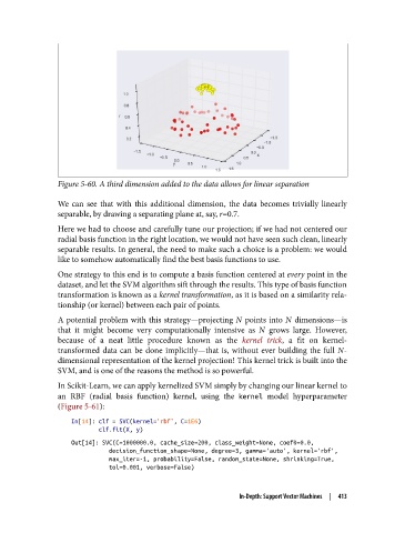
Figure 5-60. A third dimension added to the data allows for linear separation

We can see that with this additional dimension, the data becomes trivially linearly
separable, by drawing a separating plane at, say, r=0.7.

Here we had to choose and carefully tune our projection; if we had not centered our
radial basis function in the right location, we would not have seen such clean, linearly
separable results. In general, the need to make such a choice is a problem: we would
like to somehow automatically find the best basis functions to use.

One strategy to this end is to compute a basis function centered at every point in the
dataset, and let the SVM algorithm sift through the results. This type of basis function
transformation is known as a kernel transformation, as it is based on a similarity rela‐
tionship (or kernel) between each pair of points.

A potential problem with this strategy—projecting N points into N dimensions—is
that it might become very computationally intensive as N grows large. However,
because of a neat little procedure known as the kernel trick, a fit on kernel-
transformed data can be done implicitly—that is, without ever building the full N-
dimensional representation of the kernel projection! This kernel trick is built into the
SVM, and is one of the reasons the method is so powerful.
In Scikit-Learn, we can apply kernelized SVM simply by changing our linear kernel to
an RBF (radial basis function) kernel, using the kernel model hyperparameter
(Figure 5-61):

In[14]: clf = SVC(kernel='rbf', C=1E6)
clf.fit(X, y)
Out[14]: SVC(C=1000000.0, cache_size=200, class_weight=None, coef0=0.0,
decision_function_shape=None, degree=3, gamma='auto', kernel='rbf',
max_iter=-1, probability=False, random_state=None, shrinking=True,
tol=0.001, verbose=False)

In-Depth: Support Vector Machines | 413