Page 432 - Python Data Science Handbook

In[15]: plt.scatter(X[:, 0], X[:, 1], c=y, s=50, cmap='autumn')
plot_svc_decision_function(clf)
plt.scatter(clf.support_vectors_[:, 0], clf.support_vectors_[:, 1],
s=300, lw=1, facecolors='none');

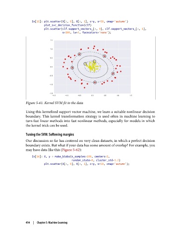
Figure 5-61. Kernel SVM fit to the data

Using this kernelized support vector machine, we learn a suitable nonlinear decision
boundary. This kernel transformation strategy is used often in machine learning to
turn fast linear methods into fast nonlinear methods, especially for models in which
the kernel trick can be used.

Tuning the SVM: Softening margins
Our discussion so far has centered on very clean datasets, in which a perfect decision
boundary exists. But what if your data has some amount of overlap? For example, you
may have data like this (Figure 5-62):

In[16]: X, y = make_blobs(n_samples=100, centers=2,
random_state=0, cluster_std=1.2)
plt.scatter(X[:, 0], X[:, 1], c=y, s=50, cmap='autumn');

414 | Chapter 5: Machine Learning