Page 436 - Python Data Science Handbook

%time grid.fit(Xtrain, ytrain)
print(grid.best_params_)
CPU times: user 47.8 s, sys: 4.08 s, total: 51.8 s
Wall time: 26 s
{'svc__gamma': 0.001, 'svc__C': 10}
The optimal values fall toward the middle of our grid; if they fell at the edges, we
would want to expand the grid to make sure we have found the true optimum.
Now with this cross-validated model, we can predict the labels for the test data, which
the model has not yet seen:
In[23]: model = grid.best_estimator_
yfit = model.predict(Xtest)
Let’s take a look at a few of the test images along with their predicted values
(Figure 5-65):

In[24]: fig, ax = plt.subplots(4, 6)
for i, axi in enumerate(ax.flat):
axi.imshow(Xtest[i].reshape(62, 47), cmap='bone')
axi.set(xticks=[], yticks=[])
axi.set_ylabel(faces.target_names[yfit[i]].split()[-1],
color='black' if yfit[i] == ytest[i] else 'red')
fig.suptitle('Predicted Names; Incorrect Labels in Red', size=14);

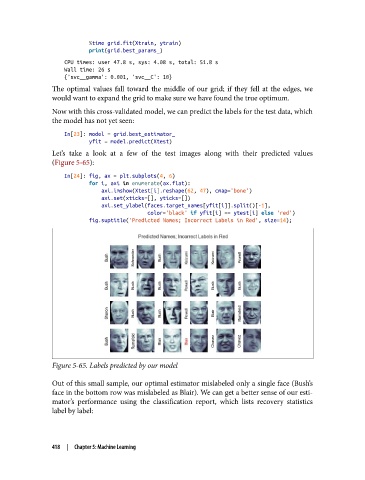
Figure 5-65. Labels predicted by our model

Out of this small sample, our optimal estimator mislabeled only a single face (Bush’s
face in the bottom row was mislabeled as Blair). We can get a better sense of our esti‐
mator’s performance using the classification report, which lists recovery statistics
label by label:

418 | Chapter 5: Machine Learning