Page 441 - Python Data Science Handbook

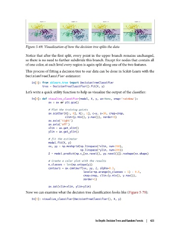
Figure 5-69. Visualization of how the decision tree splits the data

Notice that after the first split, every point in the upper branch remains unchanged,
so there is no need to further subdivide this branch. Except for nodes that contain all
of one color, at each level every region is again split along one of the two features.
This process of fitting a decision tree to our data can be done in Scikit-Learn with the
DecisionTreeClassifier estimator:
In[3]: from sklearn.tree import DecisionTreeClassifier
tree = DecisionTreeClassifier().fit(X, y)
Let’s write a quick utility function to help us visualize the output of the classifier:

In[4]: def visualize_classifier(model, X, y, ax=None, cmap='rainbow'):
ax = ax or plt.gca()

# Plot the training points
ax.scatter(X[:, 0], X[:, 1], c=y, s=30, cmap=cmap,
clim=(y.min(), y.max()), zorder=3)
ax.axis('tight')
ax.axis('off')
xlim = ax.get_xlim()
ylim = ax.get_ylim()

# fit the estimator
model.fit(X, y)
xx, yy = np.meshgrid(np.linspace(*xlim, num=200),
np.linspace(*ylim, num=200))
Z = model.predict(np.c_[xx.ravel(), yy.ravel()]).reshape(xx.shape)

# Create a color plot with the results
n_classes = len(np.unique(y))
contours = ax.contourf(xx, yy, Z, alpha=0.3,
levels=np.arange(n_classes + 1) - 0.5,
cmap=cmap, clim=(y.min(), y.max()),
zorder=1)
ax.set(xlim=xlim, ylim=ylim)
Now we can examine what the decision tree classification looks like (Figure 5-70):

In[5]: visualize_classifier(DecisionTreeClassifier(), X, y)

In-Depth: Decision Trees and Random Forests | 423